model_simple<-MCMCglmm(phen~cofactor,random=~phylo,
  family="gaussian",ginverse=list(phylo=inv.phylo$Ainv),prior=prior,
  data=data,nitt=5000000,burnin=1000,thin=500)
Here, we assume a linear relationship between
phen and
cofactor, with a random effect
phylo corresponding the
phylogenetic effect. The argument
ginverse allows us to include
a custom matrix for our random effect
phylo, using the results
of the
inverseA function (above). We used the
prior variable defined above.
The variables
nitt and
burnin
are used to calibrate the MCMCM algorithm: it will iterate for
burnin
iterations before recording samples (to ensure convergence), and then iterate
nitt times. The parameter
thin helps us to save memory by
saving only every
`thin' value and thus,
dropping highly auto-correlated values
2. Note that the use of
nodes=`TIPS' or
nodes=`ALL' in the
inverseA function can have a noticeable
impact on auto-correlation: whereas the latter would speed up computation, it
can results in higher auto-correlation. Whether to use to one or the other would
thus depend mainly on the size of the phylogeny (very large phylogenies would probably
need
nodes=`ALL' to allow MCMCglmm to run at all). Finally, note that this
example can take up to a few hours to run.
After checking for convergence (for example using heidel.diag() function),
we can look at the output summary:
##  Iterations = 1001:4999501
##  Thinning interval  = 500
##  Sample size  = 9998
##
##  DIC: 1516
##
##  G-structure:  ~phylo
##
##       post.mean l-95% CI u-95% CI eff.samp
## phylo       210     92.3      334     9998
##
##  R-structure:  ~units
##
##       post.mean l-95% CI u-95% CI eff.samp
## units      85.8     60.8      113    10986
##
##  Location effects: phen ~ cofactor
##
##             post.mean l-95% CI u-95% CI eff.samp  pMCMC
## (Intercept)     39.71    26.09    53.60     9998 <1e-04 ***
## cofactor         5.18     4.90     5.44     9998 <1e-04 ***
## ---
## Signif. codes:  0 '***' 0.001 '**' 0.01 '*' 0.05 '.' 0.1 ' ' 1
The first part shows a summary of MCMC sampling parameters, and gives the
Deviance Information Criterion (DIC) of the model. The DIC is a model selection
criterion comparable to Akaike's Information Criterion (AIC)
3. Following are the
results for the random effect variances (
G-structure, containing the variance
of the
phylo effect) and the residual variance (
R-structure,
the residual variance is called
units in MCMCglmm).
We have information about the posterior mean of
the estimate, its 95% credible interval
4
and its effective sample size. The
latter is a measure of the auto-correlation within the parameter sample: it
should be close to the MCMC sample size above, or failing that, it should be at
least large enough (say more than 1,000). The summary of the fixed
effects (
intercept and
cofactor) are similar, except we also
have a ``pMCMC'' value for significance testing if the parameter is different
from zero
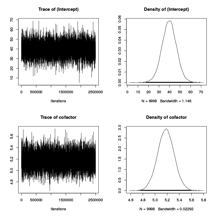
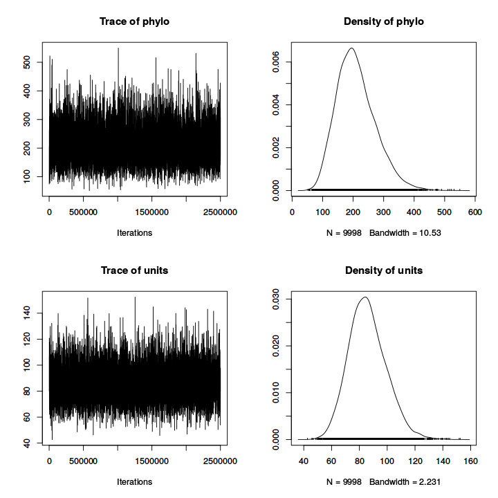
5. By
using
plot(model_simple), we can obtain the ``trace'' of the sampling
(to check for convergence and auto-correlation) and posterior density of each
parameter (Fig.
11.1).
Figure 11.1:
Plot of trace and posterior density for fixed effects (top two firsts) and
variance parameters (bottom two lasts).
|
|
Finally, we can easily calculate the posterior probability of the phylogenetic signal  (see section 11.2.1 in the main text) using:
lambda <- model_simple$VCV[,'phylo']/
 (model_simple$VCV[,'phylo']+model_simple$VCV[,'units'])
We can calculate the posterior mean (mean of the posterior distribution), posterior mode
(most likely value regarding the posterior distribution) and the 95% credible interval of
:
##       lower  upper
## var1 0.5267 0.8522
## attr(,"Probability")
## [1] 0.95
Footnotes
... 0.011
MCMCglmm univariate prior formulation
is such that it corresponds to an inverse-Gamma with shape parameter
 and scale parameter
 .
It is important to note that this inverse-Gamma could become unwantedly `informative'
when variance components are close to 0 so that it is always recommended running models with different prior specifications.
For which prior should be used, see discussion in Hadfield (2010b) and also one can find more recent discussion
on this topic online within the correspondences in the r-sig-mixed-modes mailing list.
... values2
Because the MCMC sampling is
Markovian, it is a time-series, which often appears to be auto-correlated:
closely following iterations tend to resemble each other. The ``thinning'' help
to save memory when running the MCMC for longer. For phylogenetic mixed model, this auto-correlation can be large
and problematic: always make sure your effective sample size is large enough and
that auto-correlation is low.
... (AIC)3
Here we do not
provide explanations on how information criteria can be used for model selection.
For a detailed discussion on this topic, the reader is referred to Chapter 12.
... interval4
Credible interval can be
considered as the Bayesian version of confidence intervals, and also it is
known as the highest posterior density (see Hadfield, 2010b).
... zero5
If we are strictly Bayesian, we should not do significance
testing because such a concept belongs to the frequentists' paradigm. However,
we use ``pMCMC'' as if frequentists' p-values for convenience.
.
It is important to note that this inverse-Gamma could become unwantedly `informative'
when variance components are close to 0 so that it is always recommended running models with different prior specifications.
For which prior should be used, see discussion in Hadfield (2010b) and also one can find more recent discussion
on this topic online within the correspondences in the r-sig-mixed-modes mailing list.
... values2
Because the MCMC sampling is
Markovian, it is a time-series, which often appears to be auto-correlated:
closely following iterations tend to resemble each other. The ``thinning'' help
to save memory when running the MCMC for longer. For phylogenetic mixed model, this auto-correlation can be large
and problematic: always make sure your effective sample size is large enough and
that auto-correlation is low.
... (AIC)3
Here we do not
provide explanations on how information criteria can be used for model selection.
For a detailed discussion on this topic, the reader is referred to Chapter 12.
... interval4
Credible interval can be
considered as the Bayesian version of confidence intervals, and also it is
known as the highest posterior density (see Hadfield, 2010b).
... zero5
If we are strictly Bayesian, we should not do significance
testing because such a concept belongs to the frequentists' paradigm. However,
we use ``pMCMC'' as if frequentists' p-values for convenience.