Species-specific trait data ("primate_spec.txt"), a tab separated text file, species-specific data on brain size and body size in primates, include within-species sample sizes

Phylogeny ("consensusTre_Primates.nex"), the consenus phylogenetic tree for 1000 phylogenetic hypotheses from Arnold et al. (2010), nexus format

Codes

To get started

# activate libraries
library(ape)
library(nlme)
library(AICcmodavg)
library(scatterplot3d)

# import data and tree
xdata <- read.table(file = "primate_spec.txt", header = T, sep = "\t", dec = ".")
row.names(xdata) = xdata$species
tree <- read.nexus("consensusTre_Primates.nex")

Creating different models by simultaneously varying omega (weight scaling factor) and lambda (phylogeny scaling factor)

Here we will apply multimodel inference from models relying on different lambdas and omegas. Hereafter, you are assumed to be familiar with exercises 2) and 3) within the content of this OPM.

# To make all models in two loops through different omegas and lambdas
xweights = seq(1, 0, length.out = 101)
Cand.models = list()
modnames = c()
for (l in 0:100) {
    for (w in 1:length(xweights)) {
        omega = xdata$brain_N^xweights[w]
        Cand.models[[l * 101 + w]] = gls(lg.brain ~ lg.body, data = xdata, correlation = corPagel(value = l/100,
            tree, fixed = T), weights = ~1/omega, method = "ML")
        modnames[l * 101 + w] = paste("lambda =", round(l/100, 2), ", omega =",
            round(xweights[w], 2))
    }
}

# To get model averaged estimate for the regression intercept
Int_av = modavg(parm = "(Intercept)", cand.set = Cand.models, modnames = modnames)
Int_av$Mod.avg.beta

## [1] 1.087

Int_av$Uncond.SE

## [1] 0.5398

# To get model averaged estimate for the regression slope
beta_av = modavg(parm = "lg.body", cand.set = Cand.models, modnames = modnames)
beta_av$Mod.avg.beta

## [1] 0.3033

beta_av$Uncond.SE

## [1] 0.04442

# To make figure
lambda = rep(seq(0, 1, 0.01), each = length(xweights))
omega = rep(xweights, 101)
ML = aictab(cand.set = Cand.models, modnames = modnames, sort = F)[, 7]
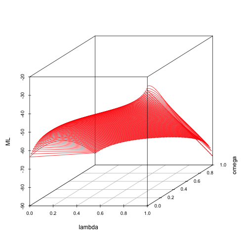
scatterplot3d(lambda, omega, ML, type = "l", color = "red")

The highest Maximum Likelihood can be found at lambda=1 and omega=0 (strong phylogenetic effect and no need to balance for differences in within-species sample sizes).

Sources

R packages

Data

Codes

To get started

Creating different models by simultaneously varying omega (weight scaling factor) and lambda (phylogeny scaling factor)

References

- Arnold C, Matthews LJ, Nunn CL (2010) The 10kTrees website: a new online resource for primate hylogeny. Evol Anthropol 19:114-118.
- Ligges U, Machler M (2003) Scatterplot3d: an R package for visualizing multivariate data. J Stat Softw 8:1-20.
- Mazerolle MJ (2013) AICcmodavg: Model selection and multimodel inference based on (Q)AIC(c). R package version 1.28.
- Paradis E, Claude J, Strimmer K (2004) APE: analyses of phylogenetics and evolution in R language. Bioinformatics 20:289-290.
- Pinheiro J, Bates D, DebRoy S, Sarkar D, R Development Core Team (2012) nlme: Linear and Nonlinear Mixed Effects Models. R package version 3.1-104,