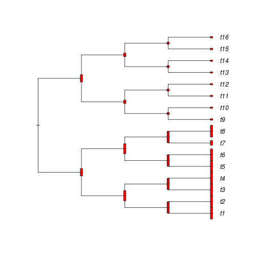
plot(ts, label.offset = 0.2) xs <- xou2/10 nodelabels(thermo = rep(1, Nnode(ts)), height = xs[-(1:16)], width = 0.05) tiplabels(thermo = rep(1, Ntip(ts)), height = xs[1:16], width = 0.05)

"ape" (Paradis et al 2004)
"geiger" (Harmon et al. 2008)
Example 1: simulating a single trait under Brownian motion
x.bm <- rTraitCont(trbd2)
x.bm
##       t1       t2       t3       t4       t5       t6       t7       t8
## -1.55583 -0.62867 -0.05259  0.18589  0.32598  1.05130  0.10769  0.28563
##       t9      t10      t11      t12      t13      t14      t15      t16
##  0.41660 -0.21336 -0.14154 -0.09060 -0.38945 -0.62948 -0.34706 -0.34775
##      t17      t18      t19      t20      t21      t22
## -0.43898 -1.52219 -0.54451 -0.38288 -0.51639 -1.25199
The BM parameter is defined by default σ = 0.1; note that this
is σ, not σ2, so this value must be squared to
calculate the expected variance with σ2T where T is the
time of evolution (which is here the age of the root because the tree is
ultrametric). The value of T can be extracted with the function
branching.times whose first value is the age of the root
and we check that this is close to the observed variance of the simulated trait:
0.1^2 * branching.times(trbd2)[1]
##  23
## 0.5
var(x.bm)
## [1] 0.3787
Example 2: contrasting continuous- and discrete-time simulation
In this exercise, we want to simulate a BM model outside a tree (which is equivalent to simulating a trait along a single branch). We will show that using a discrete-time or a continuous-time formulation give exactly the same results. We first look at the respective mathematical expressions, first in continuous time:
where N denotes the normal distribution, and in discrete time:
So it's needed to generate only one random normal variate with the
first formulation, while we need to generate T variates in the second one.
We are going to compare the running times of these two solutions in
R setting σ = 0.1 (the function rnorm is
paramerized with the standard-deviation σ while the usual
mathematical notation uses the variance σ2),
T = 100, and replicating the simulation 10,000 times (i.e., generating
10,000 values of xT):
system.time(Xcont <- rnorm(10000, 0, 1))
##    user  system elapsed
##   0.002   0.000   0.001
system.time(Xdisc <- replicate(10000, sum(rnorm(100, 0, 0.1))))
##    user  system elapsed
##   0.175   0.000   0.175
Without surprise, the continuous-time model is much faster to simulate, and, of course, this will be even worst for larger values of T. We refer to the book to compare the strengths and weaknesses of both approaches. We can test that they gave the same results by testing that the means and variances of both samples are not significantly different:
t.test(Xcont, Xdisc)
##
## 	Welch Two Sample t-test
##
## data:  Xcont and Xdisc
## t = -0.0279, df = 19998, p-value = 0.9778
## alternative hypothesis: true difference in means is not equal to 0
## 95 percent confidence interval:
##  -0.02818  0.02739
## sample estimates:
## mean of x mean of y
##  -0.01302  -0.01263
var.test(Xcont, Xdisc)
##
## 	F test to compare two variances
##
## data:  Xcont and Xdisc
## F = 1.006, num df = 9999, denom df = 9999, p-value = 0.7745
## alternative hypothesis: true ratio of variances is not equal to 1
## 95 percent confidence interval:
##  0.9671 1.0460
## sample estimates:
## ratio of variances
##              1.006
Example 3: Brownian motion with variable rate
We will take a model with random rates σ for each branch of the
tree. We use the fact that in rTraitCont, the argument
sigma can be a vector with as many values than the number of
branches of the tree. The values of σ are drawn from a
continuous distribution between 0 and 1.
sigs <- runif(Nedge(tr))
x <- rTraitCont(tr, sigma = sigs)
Example 4: Stasis with Brownian motion after speciation
The punctational model of evolution assumes that phenotypic change
occurs mainly during speciation events. We see here two ways to
simulate traits under such a model. The first one is to build a
function to be used as argument to rTraitCont (note that the
second argument of foo is not used inside the function but must
be present in its definition):
foo <- function(x, l) x + rnorm(1, 0, 0.1)
x <- rTraitCont(tr, foo)
The second way is to transform all the branch lengths to one and then
use rTraitCont in the usual way:
tr2 <- compute.brlen(tr, 1)
x <- rTraitCont(tr2)
In both cases we used σ = 0.1 and change was independent of time.
Example 5: Ornstein–Uhlenbeck model with two optima
One stength of the OU model is that the parameter θ can vary which makes possible to model variable optima in adaptive evolution. For simplicity, let's consider a fully balanced tree with n = 16 and its branch lengths set equal to one:
ts <- compute.brlen(stree(16, "b"), 1)
We then need to specify the values of θ for each branch of the tree; we choose here θ = 1 for the first half of the tree and θ = 10 for the second half (see below on how to find the indices of the branches):
theta <- rep(1, Nedge(tr))
theta[16:30] <- 10
We can now call rTraitCont with the appropriate options; we
also ask this function to output the values of the simulated trait at
the nodes of the tree:
xou2 <- rTraitCont(ts, "OU", theta = theta, ancestor = TRUE)
xou2
##     t1     t2     t3     t4     t5     t6     t7     t8     t9    t10
##  9.787  9.809  9.787  9.776  9.726  9.794  4.094  9.968  1.346  1.262
##    t11    t12    t13    t14    t15    t16  Node1  Node2  Node3  Node4
##  1.250  1.229  1.154  1.221  1.390  1.320  0.000  6.335  8.656  9.508
##  Node5  Node6  Node7  Node8  Node9 Node10 Node11 Node12 Node13 Node14
##  9.435  8.553  9.509  9.649  6.298  2.894  1.785  1.719  3.061  1.675
## Node15
##  1.700
Note that the trait value at the root (labeled Node1) is zero. We can represent these data in different ways, we choose here vertical bars after rescaling the trait values (dividing them by 10):
plot(ts, label.offset = 0.2)
xs <- xou2/10
nodelabels(thermo = rep(1, Nnode(ts)), height = xs[-(1:16)], width = 0.05)
tiplabels(thermo = rep(1, Ntip(ts)), height = xs[1:16], width = 0.05)

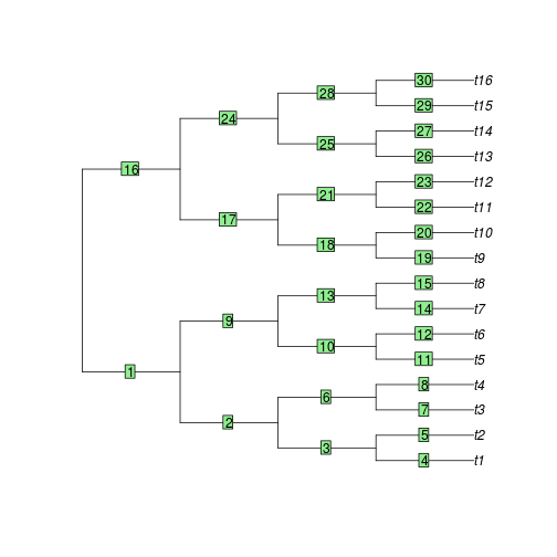
If one wants to change a specific value in the vector theta, it
is possible to find the indices of all branches with a plot of the tree:
plot(ts)
edgelabels()

Example 6: simple Markov chain
One of the simplest models of discrete trait evolution can be modeled
with a Markov chain with two states and equal transition rates. This
is the default of the function rTraitDisc:
x <- rTraitDisc(tr)
x
##  t2  t7  t5  t4 t10  t1  t3  t9  t6  t8
##   A   A   A   A   A   B   A   A   A   A
## Levels: A B
To change the model to one with asymmetric rates, we can simply use the short-cut "ARD" as model and give the values of rates (if only one value is given, an error is returned):
x <- rTraitDisc(tr, "ARD", rate = c(0.1, 0.2))
x
##  t2  t7  t5  t4 t10  t1  t3  t9  t6  t8
##   A   A   A   A   A   A   B   A   A   A
## Levels: A B
Example 7: meristic characters
This kind of discrete traits evolve so that only transitions between 'contiguous states' are possible. For instance, we can assume that the number of vertebrae (or other developmental units) can only change by adding (or removing) one vertebra at a time. There are several ways to simulate such a model of evolution in R. If the number of states is limited, it is possible to build a Markov chain where only the transitions close to the diagonal will be permitted:
m <- matrix(0, 4, 4)
for (i in 1:3) m[i, i + 1] <- m[i + 1, i] <- 2
m
##      [,1] [,2] [,3] [,4]
## [1,]    0    2    0    0
## [2,]    2    0    2    0
## [3,]    0    2    0    2
## [4,]    0    0    2    0
In this model the rates of increase and of decrease are equal, but
this can be modified easily. This matrix is then used as argument to
the option model:
rTraitDisc(tr, model = m)
##  t2  t7  t5  t4 t10  t1  t3  t9  t6  t8
##   B   A   B   B   A   B   A   B   A   A
## Levels: A B C D
This model assumes a limited number of states for the trait. For a
model with an infinite number of states, it is better to use
rTraitCont with a custom function such as:
m <- function(x, l) x + sample(-1:1, size = 1)
In this model, x is evolved by adding –1, 0, or +1 with
equal probability. These probabilities can be
changed with the option prob of sample; for instance, a
model where the probability of no change is equal to 0.9
and the probability of change in either direction is equal to 0.05
would be defined with:
m <- function(x, l) x + sample(-1:1, size = 1, prob = c(0.05, 0.9, 0.05))
Example 8: branch length transformation
We have seen several times than, under a Brownian motion model, the quantity of evolution accumulated through time is expected to be equal to σ2 T. Thus, changing the value of T (the time of evolution) will have the same effect than changing the value of σ2 (the rate of evolution) as long as their product is the same. Thus, we can simulate various models of evolution on a phylogeny by transforming its branch lengths (as long as they represent values of time).
The package geiger has the function rescale which transforms
the branch lengths of a tree according to a specified model (11 models
are available). The function compute.brlen in ape provides a
way to change branch lengths with user-defined numerical values or a
function. It is also possible to modify the length of a specific
branch in R's standard way, for instance:
tr$edge.length[5] <- 10
The transformed tree is then used to simulate traits as seen before.
Example 9: two correlated traits
There are a number of ways to model the correlated evolution of two traits. We take here a model:
where X is a vector with two values, M is a matrix giving the strength of the correlation between the two traits, and εt is a vector of two independent random normal variates. We define M as a 2 by 2 matrix with diagonal elements 1 and off-diagonal elements 0.5, which shows that this is a model with correlated errors. We can write the model as a function:
sigma <- 0.1
M <- matrix(c(1, 0.5, 0.5, 1), 2, 2)
foo <- function(x, l) x + M %*% rnorm(2, 0, sigma * l)
The function foo has the same arguments than we have seen above, but this
time it returns a vector of length two instead of a single
value. There is also a notable difference: sigma and M
have been defined outside foo and this one can found them
thanks to the lexical scoping rule of R. This is useful to run several
simulations and changing the values of these parameters as done below:
rTraitMult(tr, foo, p = 2)
##             x1       x2
## t2  -1.2441561 -2.00833
## t7  -1.3089568 -1.95362
## t5   0.2059091  0.06923
## t4   0.1045884 -0.01463
## t10 -0.1122785 -0.07383
## t1   0.1091219  0.04879
## t3  -0.2106405 -0.21023
## t9   0.0679979  0.11302
## t6   0.0610700  0.05060
## t8   0.0004179  0.02351
sigma <- 1
rTraitMult(tr, foo, p = 2)
##          x1       x2
## t2  -0.7955 -7.29234
## t7  -1.4215 -6.98234
## t5  -3.1582 -2.99656
## t4  -2.6850 -2.49535
## t10 -2.9068 -3.10976
## t1  -2.6136 -1.71306
## t3  -0.6735  0.99482
## t9  -1.4408 -0.19704
## t6  -0.4405  0.04391
## t8   0.4374 -0.66539
Example 10: assessing type I error rates
Pvalue <- function(n) {
    tr <- rtree(n)
    x <- rnorm(n)  # rTraitCont(tr)
    y <- rnorm(n)  # rTraitCont(tr)
    summary(lm(pic(x, tr) ~ pic(y, tr) - 1))$coef[1, 4]
}

typeIerrorRate <- function(n, nrep) sum(replicate(nrep, Pvalue(n)) < 0.05)/nrep

sapply(c(10, 50, 100), typeIerrorRate, nrep = 10000)
## [1] 0.1192 0.1714 0.1911
This code evaluates the type I error rate of testing the correlation
of two variables that do not evolve on a tree and controlling
(wrongly) for phylogenetic dependence. The function Pvalue can
easily be modified to simulate different scenarios (as shown after the
#). n is the number of species in the tree and
nrep is the number of replications of the simulation. The last
command was used to calculate the type I error rates reported in the
book.
Example 11: constrained simulation with a known ancestral character
This problem was suggested by Tristan Lefebure:This is a very interesting question which has many potential
applications, particularly since paleoecological data are widely
available. In the function rTraitCont, the option model
can be either "BM" or "OU", but also a function of the form
f(x, l) where x is the trait value of the ancestor
and l is the branch length; this function must return the value
of the trait after evolution along that branch. A simple example could be:
f <- function(x, l) x + rnorm(1, 0, 0.1 * sqrt(l))
rTraitCont(tr, model = f)
##       t2       t7       t5       t4      t10       t1       t3       t9
##  0.47416  0.60474  0.20600  0.27827  0.23707  0.15512  0.14326  0.24908
##       t6       t8
##  0.13863 -0.03565
which is nothing else than our classical BM model with
σ = 0.1. The way the ancestral value is called in the code of
rTraitCont makes possible to use known values for a specific
node. For instance, suppose we want to simulate a model where the
trait follows a BM process with σ = 0.1 when the variable
`habitat' is 1, and with σ = 0.5 when its is 2. To prepare our
simulations, we need to build two vectors: one with the values of
σ and one with the values of `habitat' ordered along the node
numbers of the tree:
sigma <- c(0.1, 0.5)
habitat <- c(1, 1, 2, 2)  # etc....
In this case, we would have habitat = 1 for the first and the second
nodes, etc. (the node numbering system used by ape can be displayed with
nodelabels() after plotting a tree). We can now define our
model with this function:
f <- function(x, l) {
    sig <- sigma[as.numeric(habitat[anc[i] - n])]
    x + rnorm(1, 0, sig * l)
}
The crucial bit is anc[i] which matches the internal code of
rTraitCont. Note the offset -n because the node numbers
starts from n + 1 (this offset would be omitted if habitat were a
concatenated vector of the recent and ancestral values). The
as.numeric is to insure that a numeric value is used even if
habitat is coded as a factor.