IMI data for primates ("e.dataIMI_corrected.csv"), Log10 Values of IMI and mass for 118 primate species.

Primate Phylogenies ("e.IMI.TreeBlock_10kTrees_Primates_Version3.nex"), 100 primate phylogenies sampled from 10kTrees and trimmed to species in data set.

Codes

Setup

library(ape)
library(geiger)

source(".../BayesModelS_v22.R")  #provide a path for the location of the source file that includes the functions 

treeDataAll = read.nexus("./e.IMI.TreeBlock_10kTrees_Primates_Version3.nex.txt")

data = read.csv("./e.dataIMI_corrected.csv", header=T)

factorName = c() #enter variable names here that should be treated as factors
missingList = c("Homo_sapiens") #Species listed here are exluded from model fitting, and values for response are predicted

pathO = "./"
colnames(data)

## [1] "Species"            "IMILog10"           "MassLog10"         
## [4] "Suspensory_relQuad" "VCL_relQuad"        "RadiationHap1"

formula = "IMILog10 ~ MassLog10"

Analysis

Select and check Bayesian linear model, run analysis, and predict value of unknown tip.
Input for blm function:
formula, data, treeDataAll, factorName, missingList: assigned in previous code
currentValue: sets the starting point for MCMC, default is 0. To specify a value, a list of variables should be provided
nposterior: the number of posterior draws you want. For the sake of time, this value was set to 20100 for this online example. Actual analysis performed 200100 draws
burnin, thin: the burnin rate and thin rate in the MCMC analysis. Both set to 100 for this example.
varSelection: estimates branch length scaling parameters lambda or kappa or both. Can have three values: "random" means nothing is specified and a model selection process for lambda or kappa is conducted (while simultaneously estimating the parameter selected), while "lambda" or "kappa" estimates only their respective parameters in the MCMC analysis.
lambdaUpperBound: default to 1.
kappaUpperBound: default to 1.
lambdaValue, kappaValue: this enables the user to fix the value of lambda or kappa to use in the analysis. If a value is specified, then MCMC uses this value during the MCMC analysis, rather than estimating it.
restriction: default to "no restriction". This would control whether the user wants to manually have one variable always included in the analysis, specified by name.
path: the output folder.

bmselection = blm(formula, data, treeDataAll, factorName = factorName, missingList = missingList, currentValue = 0, nposterior = 20100, burnin = 100, thin = 100, varSelection = "lambda", lambdaValue = NA, kappaValue = NA, path = pathO)

## [1] "Those species are deleted from regression"
## [1] "Homo_sapiens"
## [1] "Those species are in missingList"
## [1] "Homo_sapiens"
## [1] "pre-analysis begins..."
## [1] "pre-analysis finished, Bayesian posterior draw begins..."
## [1] "regression finished 25%"
## [1] "regression finished 50%"
## [1] "regression finished 75%"
## [1] "regression finished 100%"
## [1] "Bayesian posterior draw finished, writing files..."
## [1] "posterior sample is written in the file ./ result.csv"
## [1] "dataset is written in the file ./ data.csv"
## [1] "files writing completed..."

modelChecking(bmselection, missingList, pathO)

## [1] "initialize analysis, predictive draw begins..."
## [1] "predictive draw finished, model checking begins..."

## [1] "model checking result finished, written in file ./ modelChecking.pdf"

analysis(bmselection, path = pathO)

## [1] "initialize analysis and get posterior sample ends, analysis begins..."
## [1] "model indicator written in file ./ modelIndicator.csv"
## [1] "initial analysis completed, plot the results..."

## [1] "plot ploted in the file ./ outputBayesianModel.pdf"
## [1] "plot completed, analysis finished..."

predict(bmselection, missingList, path = pathO) #this predicts response in "missingList" species

## [1] "initialize analysis, predictive draw begins..."
## [1] "predictive draw end, begin for missing data analysis"

## [1] "missing data analysis end, begin printing out the result"

##                min 2.5%q 25%q median  mean  75%q 97.5%q   max
## Homo_sapiens 1.969 1.995 2.03  2.049 2.049 2.068  2.108 2.122

Display results

After importing the results from analysis, any number of methods can be used to display them. This example includes several possibilities

outputPosterior = read.csv("./ result.csv")

# example output for posterior sample
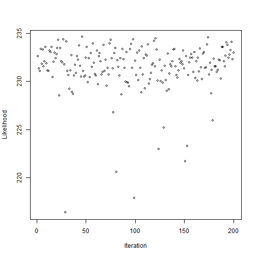
plot(outputPosterior$lkhoodSample, xlab="Iteration", ylab="Likelihood", cex=0.8, pch=1)

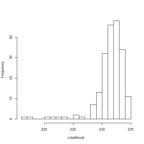
hist(outputPosterior$lkhoodSample, n=25, xlab="Likelihood", main="")

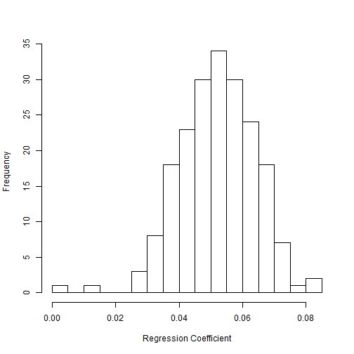
hist(outputPosterior$coef.MassLog10, xlab="Regression Coefficient", main="", n=25)

sum(outputPosterior$MassLog10)

## [1] 199

mean(subset(outputPosterior$coef.MassLog10,abs(outputPosterior$coef.MassLog10)>0) ) #mean coefficient

## [1] 0.05232

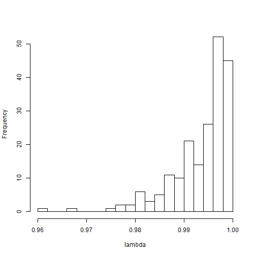
hist(outputPosterior$lambdaSample, n=20, xlab="lambda", main="")

mean(outputPosterior$lambda)

## [1] 0.9936

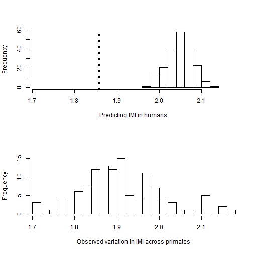
outputPosteriorHsapeiens = read.csv("./predictions.csv")

#example output for prediction distribution of value on missing tip
par(mfrow=c(2,1))
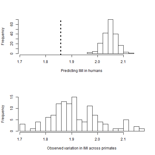
hist(outputPosteriorHsapeiens$Homo_sapiens, xlab="Predicting IMI in humans", main="", xlim=c(min(data[,2], na.rm=TRUE), max(data[,2], na.rm=TRUE)))
abline(v= data[51,2], col=1, lwd=3, lty=3)

hist(data[,2], xlab="Observed variation in IMI across primates", main="", xlim=c(min(data[,2], na.rm=TRUE), max(data[,2], na.rm=TRUE)), n=20)

Sources

R packages

Data

Codes

Setup

Analysis

Display results

References

- Paradis E., Claude J. & Strimmer K. 2004. APE: analyses of phylogenetics and evolution in R language. Bioinformatics 20: 289-290.
- Harmon Luke J, Jason T Weir, Chad D Brock, Richard E Glor, and Wendell Challenger. 2008. GEIGER: investigating evolutionary radiations. Bioinformatics 24:129-131.
- David Orme, Rob Freckleton, Gavin Thomas, Thomas Petzoldt, Susanne Fritz, Nick Isaac and Will Pearse (2013). caper: Comparative
Analyses of Phylogenetics and Evolution in R. R package version 0.5.2. http://CRAN.R-project.org/package=caper
- Arnold, C., L. J. Matthews, and C. L. Nunn. 2010. The 10kTrees Website: A New Online Resource for Primate Phylogeny. Evolutionary Anthropology 19:114-118